Basis splines

How are smooth and complex curves and curved surfaces constructed in computers for computer-aided design (CAD)? With splines!

Compared to simpler definitions such as arcs, polynomials, lines, planes, spheres and cylinders, splines allow creating smooth, complex curves and surfaces from a set of control points. Because of this, splines are unmissable in creating organic shapes in products and architecture.

Different techniques exist for contructing splines; catmull-rom splines, bezier splines, basis splines, non-uniform rational basis splines (NURBS), T-splines and more. In this article I will focus on basis splines and NURBS, as this is most commonly used in CAD software.

Note that NURBS are only a small addition to basis splines, so if you understand basis splines, you understand NURBS. We also first focus on curves, and then on surfaces.

Basis spline curve #

A basis spline curve \(C(t)\) is constructed from \(n\) control points. For each control point \(P_i\), a basis function \(B_i(t)\) is defined. These basis functions return a value between \(0.0\) and \(1.0\) for a given value of \(t\). In order to get the coordinate of basis spline curve \(C(t)\) for a value of \(t\), we multiply each basis function with their corresponding control point, and sum the result:

In other words, each basis function gives the weight with which its control point contributes to the final coordinate for a given value of \(t\).

Parameter space and coordinate space #

The basis functions \(\{B_0, B_1, \dots, B_n\}\) are in parameter space \((t)\).

Control points \(\{P_0, P_1, \dots, P_n\}\) are in coordinate space \((x, y, z)\).

Only at the final step we transform from parameter space to coordinate space by multiplying the basis functions with their corresponding control points. Before that everything happens in parameter space.

We therefore disregard coordinate space for now, and focus solely on parameter space.

Basis function #

A basis function can be understood as recursive linear interpolation; A degree \(d\) basis function is constructed from two degree \(d-1\) basis functions using the following function:

Where \(d\) is degree, \([k_0, k_1, \dots, k_{n+d+1}]\) is the knot vector and \(i\) is the index of the basis function.

The knot vector is an array of non-decreasing values (\(k_{i+1} \ge k_{i}\)) that determines the basis spline segments along the \(t\)-axis. For example, the knot vector \(k = [0, 3, 3, 5, 6]\) creates segments of length \(3, 0, 2, 1\). The length of the knot vector must be \(n + d + 1\), where \(n\) is the amount of control points or basis functions, and \(d\) is the degree of the basis function we wish to create.

The base case of the recursive function at \(d=0\) is:

The following graph shows an example recursive call chain from cubic basis function \(B_{0,3}(t)\). For brevity, we remove parameter \((t)\) in our notation. Each additional layer of recursion increases the degree of the function by \(1\), going from constant (\(d=0\)), to linear (\(d=1\)), to quadratic (\(d=2\)), to cubic (\(d=3\)).

In order to construct our cubic basis function \(B_{0, 3}\), we can work out the recursion ourselves, starting from the base cases and working our way up.

A single cubic basis function gives \(n = 1\) and \(d = 3\). So, we need a knot vector of length \(n + d + 1 = 1 + 3 + 1 = 5\). We create a uniformly spaced knot vector \(k = [0, 1, 2, 3, 4]\). This creates segments of lengths \(1, 1, 1, 1\).

Degree 0 (constant) #

First, we construct the basis functions at degree \(d = 0\).

Plotting these gives:

Note that I didn’t plot them in the same plot for clarity, but they share the same \(t\)-axis.

Degree 1 (linear) #

Then, we construct the linear basis functions \(B_{0,1}\), \(B_{1,1}\), and \(B_{2,1}\) of degree \(d = 1\).

Because the knots in our knot vector are uniformly spaced, basis functions at a given degree are simply shifted by the interval between the knots, which is \(1\) in this case. This gives:

When we fill in the values for the basis functions of degree \(d=0\), we get the following piecewise functions:

Plotting these gives:

Degree 2 (quadratic) #

Then, we construct the quadratic basis functions \(B_{0,2}\) and \(B_{1,2}\) of degree \(d = 2\):

We shift \(B_{0,2}\) by \(1\) to get \(B_{1, 2}\):

This gives the following piecewise functions:

Plotting the individual functions without clamping them gives the following plot:

And after clamping:

Degree 3 (cubic) #

Finally, we construct the cubic basis function \(B_{0, 3}\) of degree \(d=3\):

This gives the following piecewise functions:

Plotting the individual functions without clamping gives:

And after clamping:

Constructing a cubic basis spline #

Now that we know how a single cubic basis function is constructed, we can create a cubic basis spline, consisting of a set of cubic basis functions.

We create a cubic basis spline with \(6\) basis functions \(B_{0,3}\), \(B_{1,3}\), \(B_{2,3}\), \(B_{3,3}\), \(B_{4,3}\), \(B_{5,3}\), and \(B_{6,3}\). This gives \(n=7\) and \(d=3\), so we create a knot vector of size \(n+d+1=7+3+1=11\): \(k = [0, 1, 2, 3, 4, 5, 6, 7, 8, 9, 10]\), uniformly spaced for simplicity:

On the interval \(\left[k_3, k_7\right)\), this cubic basis spline forms a partition of unity: \(\sum_{i=0}^{n}B_{i,3}=1\). In other words, the sum of all basis functions for each \(t\) on that interval is \(1\). For each value of \(t\), the basis spline blends between exactly \(4\) basis functions.

To generalize, a basis spline forms a partition of unity on the interval \(\left[k_{d}, k_{n}\right)\), satisfying \(\sum_{i=0}^{n}B_{i,d}=1\), and for each value of \(t\) on that interval, it blends between exactly \(d+1\) basis functions.

Clamped basis spline #

Looking at our uniformly spaced cubic basis spline, we see that our first and last basis functions never fully go to \(1\), which means that the curve does not start and end at the corresponding first and last control point. If we want our curve to start and end at the first and last control point, we can clamp the knot vector.

This is achieved by making the first \(d+1\) knots and last \(d+1\) knots have the same value.

In the case of our cubic basis spline with \(n=7\), our knot vector becomes: \(k= [3, 3, 3, 3, 4, 5, 6, 7, 7, 7, 7]\).

Plotting this gives:

Basis function implementation in C++ #

We can implement the recursive basis function in code. Note that it can be optimized by changing the recursion into a for-loop.

 1
 2
 3
 4
 5
 6
 7
 8
 9
10
11
12
13
14
15
16
17
18

[[nodiscard]] static float basis_function(const std::vector<float>& knots,
                                          const int degree,
                                          const int i,
                                          const float t) {
  if (degree == 0) {
    return t >= knots[i] && t < knots[i + 1];
  }

  const float denominator_a = knots[i + degree] - knots[i];
  const float a = denominator_a != 0.0f ? (t - knots[i]) / denominator_a : 0.0f;
  const float basis_a = basis_function(knots, degree - 1, i, t);

  const float denominator_b = knots[i + degree + 1] - knots[i + 1];
  const float b = denominator_b != 0.0f ? (knots[i + degree + 1] - t) / denominator_b : 0.0f;
  const float basis_b = basis_function(knots, degree - 1, i + 1, t);

  return a * basis_a + b * basis_b;
}

Moving to coordinate space #

We’ve spent way too much time in parameter space \(t\). Let’s move to coordinate space \((x, y)\)!

Recall that our curve in coordinate space is defined by the following function:

Using our previously defined basis_function, we can implement \(C(t)\):

 1
 2
 3
 4
 5
 6
 7
 8
 9
10

[[nodiscard]] static float basis_spline_curve(const std::vector<float>& knots,
                                              const std::vector<float>& points,
                                              const int degree,
                                              const float t) {
  float sum = 0.0f;
  for (int i = 0; i < points.size(); ++i) {
    sum += basis_function(knots, degree, i, t) * points[i];
  }
  return sum;
}

Note that in our implementation we provide a std::vector<float>, as each component of the coordinate can be evaluated using a separate call to basis_spline_curve.

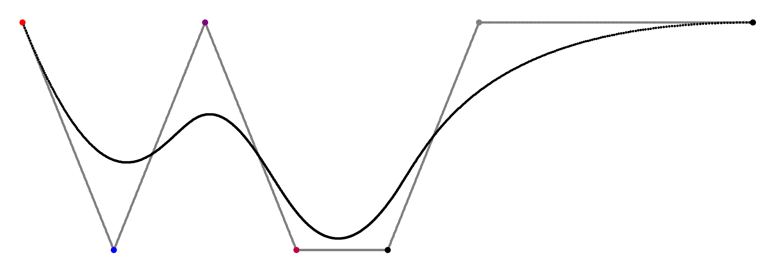
Plotting this for our clamped cubic basis spline with control points \(P = [\color{red}(0, 0)\color{black}, \color{blue}(2, 5)\color{black}, \color{#7f007f}(4, 0)\color{black}, \color{#bf013f}(6, 5)\color{black}, (8, 5), \color{gray}(10, 0)\color{black}, (16, 0)]\) gives:

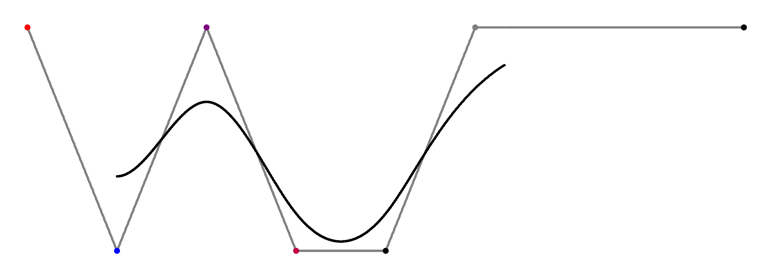
The non-clamped spline looks like this:

It’s trivial to add an additional dimension to our coordinate space:

Basis spline surfaces #

A basis spline surface \(S_d(u, v)\) with a control points matrix of size \((n \cdot m)\) is constructed by the following equation:

Where \(U_{i,d}(u)\) and \(V_{j,d}(v)\) are two separate basis splines, with their own knot vectors. As these basis splines are independent of each other, they don’t have to be of the same degree \(d\).

Let’s create a basis spline surface of degree \(d = 2\), and size \(n = 3\) and \(m = 2\).

This gives the following 2 basis splines:

• The basis spline along the \(u\)-axis, comprised of \(U_{0,2}(u)\), \(U_{1,2}(u)\) and \(U_{2,2}(u)\).
• The basis spline along the \(v\)-axis, comprised of \(V_{0,2}(v)\) and \(V_{1,2}(v)\).

The \(U_{i,d}(u) V_{j,d}(v)\) part in the equation is also known as the tensor product or outer product of the two basis splines. The tensor product of our two basis splines gives the following 2D basis functions \(B_{i, j}(u, v)\) (we remove the degree \(d\) from the subscript for brevity):

• \(B_{0, 0}(u, v) = U_{0}(u)V_{0}(v)\)
• \(B_{1, 0}(u, v) = U_{1}(u)V_{0}(v)\)
• \(B_{2, 0}(u, v) = U_{2}(u)V_{0}(v)\)
• \(B_{0, 1}(u, v) = U_{0}(u)V_{1}(v)\)
• \(B_{1, 1}(u, v) = U_{1}(u)V_{1}(v)\)
• \(B_{2, 1}(u, v) = U_{2}(u)V_{1}(v)\)

Plotting these gives:

Each individual 2D basis function \(B_{i, j}(u, v)\) corresponds to a single control point \(P_{i, j}\) in our control point matrix. For our basis spline surface, our control point matrix has the following shape:

The control point gets multiplied with its corresponding 2D basis function for a given value of \(u\) and \(v\) to get the amount with which that control point contributes to the final coordinate.

If we evaluate our basis functions for \(u=3\) and \(v=2\), we get:

For \(u=1.5\) and \(v=2.5\), we get:

Filling this into \(S(u, v)\) gives:

In code this becomes:

 1
 2
 3
 4
 5
 6
 7
 8
 9
10
11
12
13
14
15
16
17
18
19
20
21
22
23

// control points are stored in row-major format
float basis_spline_surface(const std::vector<float>& knots_u,
                           const std::vector<float>& knots_v,
                           const std::vector<float>& control_points,
                           const int rows,
                           const int columns,
                           const int degree,
                           const float u, 
                           const float v) {
  float sum = 0.0f;

  for (int row = 0; row < rows; ++row) {
    for (int column = 0; column < columns; ++column) {
      const float basis_u = basis_function(knots_u, degree, column, u);
      const float basis_v = basis_function(knots_v, degree, row, v);
      const float control_point = control_points[row * columns + column];

      sum += basis_u * basis_v * control_point;
    }
  }

  return sum;
}

Similar to the basis_spline_curve function, each component can be evaluated separately, so we provide a std::vector<float> for the control points, instead of std::vector<vec3>.

This video shows the basis_spline_surface function in action. The title of the video secretly already hints at that basis splines and NURBS are essentially the same thing.

Limitations of basis spline surfaces #

One major limitation of basis spline surfaces is that the control point topology must be a rectangular grid. This has the result that forming more complex mesh topologies requires creating separate surface “patches”, and aligning them as closely as possible. Gaps and intersections are inevitable with this approach, so for downstream applications of meshes made out of basis spline surface patches, various mesh-cleanup algorithms are devised. T-splines alleviate the topology limitation by allowing T-junctions in the parameter-space control point mesh topology. However, constructing T-splines is quite involved so they warrant their own article.

Non-uniform rational basis splines (NURBS) #

Non-uniform rational basis splines, or NURBS for short, are basis splines. Just with two properties explicitly specified:

Non-uniform #

The non-uniform part in the term means that the knot vector does not have equally spaced knots. This gives the user more control over the resulting curve.

As an effect, multiple knots can be placed at exactly the same value for \(t\), which can break curve continuity. Clamping the basis spline in the manner discussed earlier also requires creating a non-uniform knot vector.

Rational #

The rational part in the term means that we add a fourth component to our coordinate space: \(w\). The result from our spline function \(C(t)\) then returns a 4D coordinate: \(P(xw, yw, zw, w)\). In order to get our point in 3D \((x, y, z)\), we divide each component by \(w\):

These 4D coordinates are also known as homogeneous coordinates. Dividing by \(w\) can be thought of as projecting the point from 4D onto the 3D hyperplane at \(w = 1\).

While that sounds complicated, in practice it’s easiest to think about the \(w\) component as the “weight” of a specific control point, as it makes the control point “pull” harder on the curve or surface.

Conclusion #

In this article I hope to have demystified basis splines a bit and have been able to convey their beauty. I have compiled a short list of my key takeaways:

• Basis splines are just recursive linear interpolation.
• NURBS are just basis splines with a more intimidating name.
• Just focus on parameter space, coordinate space is only the final step.
• Basis spline surfaces are constructed using two completely independent basis splines.
• Solving the recursion formula yourself is not that hard, and shows the beauty of how the tangent of the two polynomials exactly aligns at a knot.

I only focused on how to construct basis spline curves and surfaces, but there are of course more things to learn about and do with them! Some potential directions to dive into:

• Solving surface-surface intersections numerically
• Showing why solving surface-surface intersections analytically is insane (due to the high degree of the resulting polynomials).
• Solving surface-curve intersections numerically
• Inserting control points without changing the overall curve (local refinement)
• Curve-fitting algorithms
• Closed-loop curves
• How to project control points onto the curve / surface itself, and inferring the new actual control points from this updated projected control point
• Tessellation of a basis spline surface that takes into account the curvature of the surface, instead of sampling the surface at a fixed interval
• Construction of certain shapes, such as bevels, cylinders and spheres using just NURBS
• Visualizing and ensuring curve continuity
• NURBS patch alignment and continuity requirements
• Cleaning up NURBS geometry for downstream applications such as FEM

Some excellent reading material about NURBS:

• The NURBS Book by Les A. Piegl, Wayne Tiller
• CS3621 Introduction to Computing with Geometry Notes by Dr. C.-K. Shene: https://pages.mtu.edu/~shene/COURSES/cs3621/NOTES/